Apache spark is a General-purpose, in-memory compute engine. It is a plug-and-play compute engine - we can plug spark with any storage system(S3, Local storage, HDFC etc..) and any resource manager(YARN, Kubernetes, Mesos, etc). Spark on top of Hadoop(Spark + hadoop + YARN) is the current industry trend.

Official documentatation:-

spark.apache.org/docs/latest/rdd-programmin..

Spark Context:-

Spark Context, also known as SparkContext, is a key component of Apache Spark, an open-source distributed computing framework. It acts as the entry point and connection to a Spark cluster. Spark Context manages the execution of tasks, coordinates resources, and provides interfaces for interacting with Spark. It allows you to create and manipulate distributed datasets (RDDs), executes Spark jobs, manages cluster resources, and facilitates interaction with external storage systems. In essence, Spark Context is the foundational component that enables distributed data processing in Spark applications.

Resilient Distributed Dataset(RDD):-

RDD (Resilient Distributed Datasets) is a fundamental data structure in Apache Spark. RDDs are immutable distributed collections of objects, partitioned across nodes in a cluster and can be processed in parallel.

RDDs can be created from different sources such as local collections, Hadoop Distributed File System (HDFS), and external storage systems such as Amazon S3, Cassandra, and HBase. Once created, RDDs can be transformed into new RDDs using various transformations such as map, filter, and reduce, and can be persisted in memory for faster access.

RDDs are fault-tolerant, meaning that they can automatically recover from node failures by recomputing lost partitions using a lineage graph.

Immutability of RDD:-

RDDs (Resilient Distributed Datasets) are immutable, which means that once an RDD is created, its contents cannot be modified. This immutability property has several important implications for Spark applications.

Data Consistency: Since RDDs are immutable, any operation that modifies an RDD creates a new RDD with the modified contents. This ensures that the original data is not modified, which is important for maintaining data consistency and ensuring reproducibility.

Fault Tolerance: The immutability of RDDs is a fundamental component of Spark's fault-tolerance mechanism. If a node in a cluster fails, Spark can recover the lost data partitions by re-executing the transformations on the RDDs that depend on the lost partitions. This is possible because the original RDDs are immutable and the lineage graph tracks the dependencies between RDDs.

Optimization: The immutability of RDDs enables Spark to optimize the execution plan of a Spark application by allowing Spark to cache intermediate results and reuse them across multiple stages. This is possible because the intermediate results are immutable and can be safely reused without any risk of data corruption.

Directed Acyclic Graph:-

DAG (Directed Acyclic Graph) is a fundamental concept in Spark's execution model, used to represent the logical execution plan of a Spark application. The DAG is a directed graph of stages, where each stage represents a set of tasks that can be executed in parallel.

When a user submits a Spark job, Spark converts the job into a DAG of stages, where each stage corresponds to a set of transformations that can be executed in parallel. The DAG is created by analyzing the dependencies between the RDDs and the transformations applied to them.

The DAG is divided into two types of stages:- Narrow stages and Wide stages. Spark uses the DAG to optimize the execution plan of the application by grouping together transformations that can be executed in a single stage, and minimizing the number of shuffles needed. By analyzing the DAG, Spark can also optimize the partitioning of the data to minimize data movement and improve performance.

Lineage Graph:-

The lineage graph is a directed acyclic graph (DAG) that represents the dependencies between RDDs (Resilient Distributed Datasets) in a Spark job. Each RDD in the lineage graph is represented as a node, and the edges between the nodes represent the transformations that were used to derive one RDD from another. The lineage graph is used to recover lost RDD partitions in case of node or process failures.

When a new RDD is created as a result of a transformation on one or more parent RDDs, Spark adds the new RDD to the lineage graph as a new node, and creates an edge from each parent RDD to the new RDD. This edge represents the dependency of the new RDD on its parent RDDs. This process is repeated for each RDD in the job, resulting in a DAG that represents the entire computation.

For a child RDD in the lineage graph, the edges leading to it represent the transformations that were used to derive it from its parent RDDs. The child RDD can only be computed after its parent RDDs have been computed, so the child RDD depends on its parent RDDs. The lineage graph ensures that all parent RDDs are computed before the child RDD is computed and that the computation is executed in the correct order.

The lineage graph is an important feature of Spark because it allows Spark to recover from node or process failures. If a node fails, Spark can use the lineage graph to determine which RDD partitions were lost, and then recompute those partitions using the remaining partitions and the transformations in the lineage graph. This ensures that the job can continue even in the face of failures.

DAG vs Lineage Graph:-

The lineage graph and the DAG (Directed Acyclic Graph) are related concepts in Apache Spark, but they are not exactly the same thing.

The lineage graph is a directed acyclic graph (DAG) that represents the dependencies between RDDs (Resilient Distributed Datasets) in a Spark job. Each RDD in the lineage graph is represented as a node, and the edges between the nodes represent the transformations that were used to derive one RDD from another. The lineage graph is used to recover lost RDD partitions in case of node or process failures.

On the other hand, the DAG is a more general concept that refers to any directed graph with no cycles. In Spark, the term DAG is often used to refer to the execution plan of a Spark job. The execution plan is a DAG that represents the stages of the job and the dependencies between them.

The lineage graph is a specific type of DAG that is used to represent the dependencies between RDDs in a Spark job. The lineage graph is a DAG because it has no cycles, and it is directed because the edges represent the direction of data flow between the RDDs. However, the lineage graph is only a part of the overall DAG of a Spark job, which includes not only the lineage of RDDs but also other stages and dependencies between stages.

In summary, the lineage graph is a specific type of DAG that represents the dependencies between RDDs in a Spark job, while the DAG is a more general concept that refers to any directed graph with no cycles. The lineage graph is a part of the overall DAG of a Spark job, but it does not include all the stages and dependencies in the job.

Types of operations in spark:-

Transformations:

Transformations are operations that transform one RDD into another RDD. However, they do not compute any result immediately but rather build a new RDD that describes how to compute the data. The transformed RDDs are lazily evaluated, meaning that the computation is deferred until an action is called on the RDD. Some common transformations in Spark include:

map: applies a function to each element of an RDD and returns a new RDD.

filter: returns a new RDD containing only the elements that satisfy a given predicate.

flatMap: applies a function to each element of an RDD and returns a new RDD that contains the concatenated results.

flatMapValues:- Applies a function to each value in a key-value pair, producing a sequence of zero or more new key-value pairs for each original key-value pair. The resulting collection is then flattened into a single collection.

groupByKey: groups the values of an RDD that have the same key into a single sequence.

reduceByKey:- It aggregates the values of each key using a specified function and returns a new RDD with the reduced values for each key.

Actions:

Actions are operations that trigger the computation of the RDD and return a result to the driver program or write data to an external storage system. When an action is called, Spark computes the RDD lineage, which is the sequence of transformations that were applied to the RDD to get to the result. Some common actions in Spark include:

collect: returns all the elements of an RDD to the driver program as an array.

reduce: aggregates the elements of an RDD using a given function.

count: returns the number of elements in an RDD.

countByValue:- counts the frequency of each unique element in the RDD and returns the result as a Map.

saveAsTextFile: writes the elements of an RDD to a text file.

Narrow Transformations vs wide Transformations:-

Narrow transformations are transformations that can be executed on a single partition of the dataset without the need to shuffle or exchange data with other partitions. Examples of narrow transformations include map, filter, and union.

Wide transformations are transformations that require data to be shuffled and exchanged between partitions. These transformations involve the aggregation, grouping or sorting of data across multiple partitions. Examples of wide transformations include reduceByKey, groupByKey, and join.

The main difference between the two types of transformations is that narrow transformations can be executed in parallel across all partitions, whereas wide transformations require communication between the nodes in the cluster to aggregate data across partitions.

It's important to note that wide transformations are more expensive than narrow transformations in terms of time and resources, as they require additional data movement and coordination across the nodes in the cluster. As such, minimizing the use of wide transformations can help to improve the performance and scalability of Spark applications.

Stages in Spark:-

Stages are marked by shuffle boundaries i.e a new stage gets created whenever we encounter a shuffle or wide transformation. The stages in Spark can be categorized as either shuffle or non-shuffle stages, depending on whether they involve data shuffling or not.

Non-Shuffle Stages:

A non-shuffle stage is a stage that does not involve data shuffling, and it can be executed entirely within a single node in the cluster without the need to transfer data between nodes. Examples of non-shuffle stages include filtering, mapping, and reducing operations that can be applied to each partition of the dataset independently.

Shuffle Stages:

A shuffle stage is a stage that involves data shuffling, and it requires data to be redistributed across the cluster based on specific keys. This is an expensive operation in terms of network and I/O overhead, and it requires coordination among multiple nodes in the cluster. Examples of shuffle stages include operations like groupByKey and join that require data to be reorganized based on keys and redistributed across the cluster.

redyceByKey vs reduce:-

reduceByKey is a wide transformation that groups the values for each key in an RDD and then applies a reduce function to the values of each group. It returns a new RDD with the same keys and the reduced values. The reduceByKey operation is a transformation because it does not actually compute a result; it only creates a new RDD with the necessary information to perform the computation.

reduce is an action that applies a binary operator to elements of an RDD and returns a single value. This single value is a local variable in the driver program. It does not group elements by key and can only be used to aggregate data without grouping by key. The reduce operation is an action because it triggers the actual computation of the reduction.

groupbyKey vs reduceByKey:-

groupbykey and reducebykey will fetch the same results. However, there is a significant difference in the performance of both functions. reduceByKey() works faster with large datasets than groupByKey()

In reduceByKey(), data partitions on the same machine with the same key are combined before the data is shuffled. So, the data is already reduced at the node level. It is then shuffled where it is then reduced at the cluster level. This reduces the overall Network IO.

In groupByKey(), all the key-value pairs are shuffled across the network. This is a lot of unnecessary data to transfer over the network. Hence, it is a more expensive operation than reduceByKey()

Note:- groupBykey can lead to 'out of memory' errors in Spark, especially when dealing with large datasets. The reason for this is that groupBykey creates a new RDD that contains all the values associated with each key in the original RDD. If the number of unique keys in the RDD is very large or if the values associated with each key are themselves very large, the resulting RDD may not fit in memory and can cause 'out of memory' errors.

Predicate pushdown:-

phpfog.com/what-is-predicate-pushdown

Predicate pushdown is a performance optimization technique used in Apache Spark to improve query execution performance in data processing tasks. It involves pushing down filtering conditions to the data sources (e.g., Hadoop HDFS, Hive, etc.) to reduce the amount of data that needs to be processed.

In Spark, predicate pushdown is supported for both relational and non-relational data sources. When using Spark SQL to query data sources, Spark's optimizer attempts to push down the filters to the data sources. This is done by converting the filter expressions into query expressions that can be evaluated directly by the data sources.

For example, suppose you have a large dataset stored in Hadoop HDFS, and you want to query the data to retrieve all records where the value of a certain column is greater than a specified value. If you were to load the entire dataset into memory in Spark and then apply the filter, it would be a very inefficient operation. However, if the filtering condition is pushed down to the HDFS storage layer, then only the relevant data is retrieved, which greatly improves query performance.

To enable predicate pushdown in Spark, you can use the pushdown method when reading data from a data source. For example, when reading data from a Hive table, you can enable predicate pushdown as follows:

COPY

spark.read.format("hive").option("pushdown", "true").load("my_table")

Broadcast variable:-

In Apache Spark, a broadcast variable is a read-only variable that is cached on each machine in the cluster instead of being sent over the network for each task. This can greatly improve the performance of Spark jobs that require the use of large read-only data sets.

Broadcast variables are created using the SparkContext.broadcast() method, which takes a value as an argument and returns a Broadcast object. This object can be used in Spark operations that require access to the broadcast value.

For example, suppose you have a large lookup table that you want to use in a Spark job. You could create a broadcast variable for this table as follows:

COPY

lookup_table = {"key1": "value1", "key2": "value2", ...}
broadcast_table = sc.broadcast(lookup_table)

Once the broadcast variable is created, you can use it in Spark operations as follows:

COPY

rdd = sc.parallelize(data)
result = rdd.map(lambda x: broadcast_table.value.get(x, None)).collect()

Accumulator variable:-

In Apache Spark, an accumulator is a shared variable that can be used to accumulate values across multiple tasks in a distributed environment. An accumulator is used to implement counters and sums in Spark applications.

Accumulators are defined on the driver program and are initialized to a default value. These accumulators are then used as read-only variables by tasks running on worker nodes. Tasks running on worker nodes can only add values to an accumulator. They cannot read or modify the value of the accumulator.

The values of accumulators are only sent to the driver program when an action is triggered, such as calling the count() method on an RDD. Spark ensures that the values are accumulated correctly even when tasks are executed in parallel across multiple worker nodes.

YARN - Yet Another Resource Negotiator:-

Resource management in MR1:-

Job Tracker and Task Tracker:-

The JobTracker and TaskTracker are components of MapReduce 1 (also known as "Classic MapReduce"), which is an older version of the MapReduce framework that is now deprecated. They play a critical role in the processing of data.

The JobTracker is responsible for managing all the jobs submitted to the Hadoop cluster. It tracks the progress of each job, manages resources, and schedules tasks on TaskTrackers. The JobTracker also monitors the health of the TaskTrackers and reallocates tasks in case of failures. It ensures that the data is processed in a fault-tolerant and efficient manner.

On the other hand, the TaskTracker is responsible for executing individual tasks that are assigned to it by the JobTracker. Each TaskTracker runs on a separate node in the cluster and is responsible for executing a subset of the tasks in a job. The TaskTracker communicates with the JobTracker to get its task assignments and to report the status of the tasks as they are completed.

In summary, the JobTracker manages and schedules jobs and tasks across the cluster, while the TaskTracker executes the tasks on individual nodes and reports their progress back to the JobTracker. Together, these two components enable MapReduce to process large amounts of data in a distributed and fault-tolerant manner.

Limitations:-

Limited Scalability:- MR1 has a fixed-size cluster architecture, which means that the cluster used by MapReduce version 1 (MR1) is composed of a fixed number of nodes. In other words, the size of the cluster is determined when the cluster is first set up and cannot be changed dynamically. Each node in the cluster serves as both a data node and a task tracker. This fixed-size cluster architecture has certain implications. For example, it can make it difficult to scale the cluster to handle larger amounts of data or more complex jobs. Additionally, since multiple jobs may compete for the same set of nodes, the cluster can be prone to resource contention.

Fixed number of Map and Reduce slots: MapReduce 1 has a fixed number of map and reduce slots per node, which is determined during the configuration of the cluster. This fixed number can limit the number of concurrent map and reduce tasks that can run on a node, leading to underutilization of resources and potentially slow processing times.

Limited support for real-time processing: MapReduce 1 is designed for batch processing of large datasets, and it lacks the ability to process data in real-time. This means that it is not suitable for applications that require real-time processing or near real-time processing.

Single-point-of-failure: MapReduce 1 has a single point of failure, which is the JobTracker. If the JobTracker fails, the entire job fails, and the processing must be restarted from scratch.

Inefficient for small data sets: MapReduce 1 is not efficient for processing small datasets. The overhead of setting up a MapReduce job is relatively high compared to the processing time, making it unsuitable for small data sets.

Difficulty in handling iterative algorithms: MapReduce 1 has difficulty handling iterative algorithms, such as machine learning algorithms, which require repeated processing of the same data set.

Limited support for complex data types: MapReduce 1 has limited support for complex data types such as graphs, trees, and matrices.

Lack of support for data partitioning: MapReduce 1 lacks support for data partitioning, which can lead to uneven workload distribution and slow down processing.

Limited fault tolerance: MapReduce 1 has limited fault tolerance capabilities, and if a node fails during processing, the entire job may fail.

YARN (Yet Another Resource Negotiator) was introduced in Hadoop 2.0 to overcome the limitations of the previous MapReduce-only architecture:-

YARN architecture is based on the concept of a global ResourceManager (RM) and per-application ApplicationMaster (AM). The ResourceManager and ApplicationMaster components are responsible for managing cluster resources and coordinating the execution of applications respectively.

The YARN architecture consists of the following components:-

ResourceManager (RM): The ResourceManager is the central authority that manages the cluster's resources and schedules the resources for the application. It consists of two main components, the Scheduler and the Applications Manager. The Scheduler is responsible for allocating resources to running applications, while the Applications Manager is responsible for accepting job submissions, negotiating the first container for executing the application-specific ApplicationMaster, and providing a tracking interface to the client.

NodeManager (NM): The NodeManager is responsible for managing resources available on a single node in the cluster. It is responsible for launching and monitoring containers on a node, managing the lifecycle of containers, and reporting the status of the containers to the ResourceManager.

ApplicationMaster (AM): The ApplicationMaster is responsible for managing the execution of an application. It is specific to a single application and is launched by the ResourceManager on a container. Once launched, it negotiates resources with the ResourceManager, requests containers from the NodeManager, and monitors the application's progress.

Container: The Container is a lightweight process that executes a specific task within an application. It represents a specific allocation of resources (CPU, memory, etc.) on a node in the cluster.

Uberization/uber mode:-

"Uber mode" is a feature in YARN that allows a single application to run entirely within a single container, rather than spreading its tasks across multiple containers in a distributed cluster.

The purpose of the Uber mode is to simplify the development and testing of applications by allowing them to be run on a single node, without the need for a full Hadoop cluster. This can be useful for developers who are working on applications that only require a small amount of data and processing power, or for testing and debugging purposes.

In Uber mode, the Application Master and the tasks it manages are run within a single container on a single node, rather than being distributed across multiple nodes in the cluster. This allows the application to be executed without the need for a fully-configured Hadoop cluster, reducing the development and testing time.

However, it is important to note that Uber mode is not intended for production use, as it does not take advantage of the scalability and fault-tolerance features of YARN. Applications that are run in Uber mode are limited to the resources available on a single node, which may not be sufficient for larger-scale applications. Therefore, Uber mode should be used only for development and testing purposes.

Spark on YARN architecture:-

In Spark on YARN architecture, there are two deployment modes: client mode and cluster mode.

sujithjay.com/spark/with-yarn

blog.knoldus.com/understanding-how-spark-ru..

sc.defaultParallelism:

sc.defaultParallelism is a configuration parameter in Spark that determines the default number of partitions that Spark will use when parallelizing data across a cluster. It specifies the number of tasks that can run in parallel in a single Spark job.

The default value of sc.defaultParallelism is typically set to the number of cores available on the cluster, although it can be configured to a different value based on the specific requirements of the application. For example, if you have a cluster with 16 cores, the default value of sc.defaultParallelism would be 16.

The number of partitions can have a significant impact on the performance of Spark jobs, as it affects the degree of parallelism in data processing. In general, having a larger number of partitions can improve the performance of Spark jobs by enabling more parallelism, but it can also result in higher overhead and communication costs between nodes.

To optimize the value of sc.defaultParallelism, it is important to consider factors such as the size of the dataset, the available resources on the cluster, and the nature of the data processing tasks involved in the job. In some cases, it may be beneficial to adjust the value of sc.defaultParallelism to achieve better performance.

rdd.getNumPartitions:-

getNumPartitions is a method in Spark that returns the number of partitions of an RDD (Resilient Distributed Dataset) or DataFrame. Partitions are the fundamental units of parallelism in Spark and represent a logical division of the data in a distributed dataset.

The getNumPartitions method can be used to check how many partitions an RDD or DataFrame is currently divided into. This can be useful for optimizing the performance of Spark jobs, as it allows you to tune the number of partitions to best fit the characteristics of the data and the available resources on the cluster.

For example, if you have a very large RDD and you find that it is taking a long time to process, you can use getNumPartitions to determine how many partitions the RDD is currently divided into. If the number of partitions is too small, you can increase it using the repartition method to improve parallelism and optimize performance. Similarly, if you have a small RDD with too many partitions, you can use the coalesce method to reduce the number of partitions and minimize overhead.

In summary, getNumPartitions is a useful method in Spark for understanding the current partitioning of RDDs or DataFrames and optimizing the performance of Spark jobs.

sc.defaultMinPartitions:-

sc.defaultMinPartitions is a configuration parameter in Spark that determines the minimum number of partitions that Spark will create when reading data into an RDD (Resilient Distributed Dataset) from a file.

By default, sc.defaultMinPartitions is set to 2. When reading data from a file, Spark will use this value as the minimum number of partitions, even if the input file is smaller than the default value. This can be useful for ensuring that the data is properly partitioned and distributed across the cluster for efficient processing.

It's worth noting that the actual number of partitions created by Spark when reading data from a file depends on various factors, such as the size of the input file and the available resources on the cluster. Spark will attempt to create a reasonable number of partitions based on the input size and available resources.

You can adjust the value of sc.defaultMinPartitions to suit the requirements of your application. For example, if you are working with a large input file and you want to ensure that the data is partitioned and distributed more finely, you can increase the value of sc.defaultMinPartitions. Conversely, if you are working with a smaller input file and you want to reduce overhead, you can decrease the value of sc.defaultMinPartitions.

rdd.repartition:-

In Spark, we can use the repartition method to repartition an RDD with a new number of partitions. It involves shuffling the data across the cluster to create new partitions, which can be useful for optimizing the performance of Spark jobs.

If we have an RDD with too few partitions, we can use repartition to increase the number of partitions and enable more parallelism. Similarly, if we have an RDD with too many partitions, we can use repartition to reduce the number of partitions and minimize overhead.

The repartition method can be called with a single argument, which specifies the desired number of partitions for the RDD. For example, rdd.repartition(10) will repartition the RDD into 10 partitions.

However, it's important to keep in mind that repartitioning can be an expensive operation, as it involves shuffling(hence a wide transformation) the data across the network. Therefore, we should use repartition judiciously and only when it's necessary to optimize the performance of Spark jobs. In some cases, other methods such as coalesce or partitionBy may be more appropriate for optimizing partitioning without the need for shuffling the data.

rdd.coalesce:-

In Spark, the coalesce method is used to reduce the number of partitions in an RDD (Resilient Distributed Dataset) without shuffling the data. This method is useful when we want to reduce the number of partitions in an RDD to optimize the performance of our Spark job.

The coalesce method can be called with a single argument, which specifies the desired number of partitions for the RDD. For example, rdd.coalesce(2) will reduce the number of partitions in the RDD to 2. Unlike the repartition method, coalesce does not involve shuffling the data across the network, so it is a more efficient way to reduce the number of partitions in an RDD.

However, it's important to note that the coalesce method can only be used to reduce the number of partitions in an RDD. If we want to increase the number of partitions, we need to use the repartition method.

In summary, the coalesce method in Spark is a useful way to reduce the number of partitions in an RDD without shuffling the data. By using it appropriately, we can optimize the performance of our Spark jobs without incurring the overhead of shuffling data across the network.

coalesce vs repartition:-

coalesce and repartition are both methods in Spark that can be used to control the partitioning of RDDs. However, there are some differences between the two methods that are important to note.

repartition involves shuffling the data across the network to create a new set of partitions with a desired number. This can be an expensive operation, especially if the number of partitions is significantly increased or decreased.

On the other hand, coalesce allows us to reduce the number of partitions without shuffling the data, as long as we specify a smaller number of partitions than the original RDD. coalesce can be thought of as a "lazy" version of repartition because it tries to minimize the amount of data movement across the network. However, it's important to note that coalesce only merges adjacent partitions, so it cannot be used to increase the number of partitions.

Another difference between the two methods is that repartition can be used to both increase and decrease the number of partitions, while coalesce can only be used to decrease the number of partitions. If we want to increase the number of partitions using coalesce, we would need to first use repartition to increase the number of partitions, and then use coalesce to reduce the number of partitions to the desired amount.

In terms of performance, coalesce can be faster than repartition when we only need to reduce the number of partitions because it avoids the costly shuffling operation. However, when we need to significantly increase or decrease the number of partitions, repartition may be faster because it can perform the data movement in parallel across the network.

In summary, coalesce and repartition are both methods for controlling the partitioning of RDDs in Spark, but they have some differences in their behavior and performance. coalesce is a "lazy" method that only merges adjacent partitions and is useful for reducing the number of partitions, while repartition can both increase and decrease the number of partitions, but can be expensive when significant data movement is required.

Serialized and non-serialized storage:-

Serialized and non-serialized storage are two different ways of storing data in a computer system. Serialized storage refers to a storage mechanism where data is converted into a stream of bytes before storing it on disk or transmitting it over a network. This means that the data is transformed into a binary format, which can be more compact and efficient for storage and transmission. However, the data cannot be directly read or modified by humans because it is not in a human-readable format.

Non-serialized storage, on the other hand, stores data in a format that can be directly read and modified by humans. Examples of non-serialized storage include text files, images, videos, and audio files. Non-serialized storage is typically used when human readability is required, or the data is not suitable for serialization due to its complex structure or size.

In the context of big data processing frameworks like Apache Spark, serialization plays an essential role in improving performance by reducing the amount of data that needs to be transmitted over the network or stored on disk. Spark uses a binary serialization format called Apache Avro for efficient storage and transmission of data. Avro can encode and decode data more quickly than text-based formats like JSON or CSV, resulting in faster data processing.

In Spark, users can choose between serialized and non-serialized storage when caching or persisting data. Serialized storage can be more memory-efficient, but it requires additional time to serialize and deserialize the data. Non-serialized storage, on the other hand, is slower but provides more human-readable data for debugging or troubleshooting. By default, Spark uses serialized storage for caching and persisting data. However, users can specify the storage format by providing a serialization codec or format when caching or persisting RDDs or DataFrames.

Cache and persist:-

In Apache Spark, caching and persisting are two mechanisms for optimizing data processing by storing data in memory or disk for faster access.

Caching:-

Caching is an in-memory data storage mechanism that allows Spark to persist frequently accessed RDDs (Resilient Distributed Datasets) or DataFrames in memory so that subsequent operations can be executed more quickly. By default, Spark caches data in memory, but it can also spill the data to disk if there is not enough memory available.

Persist:-

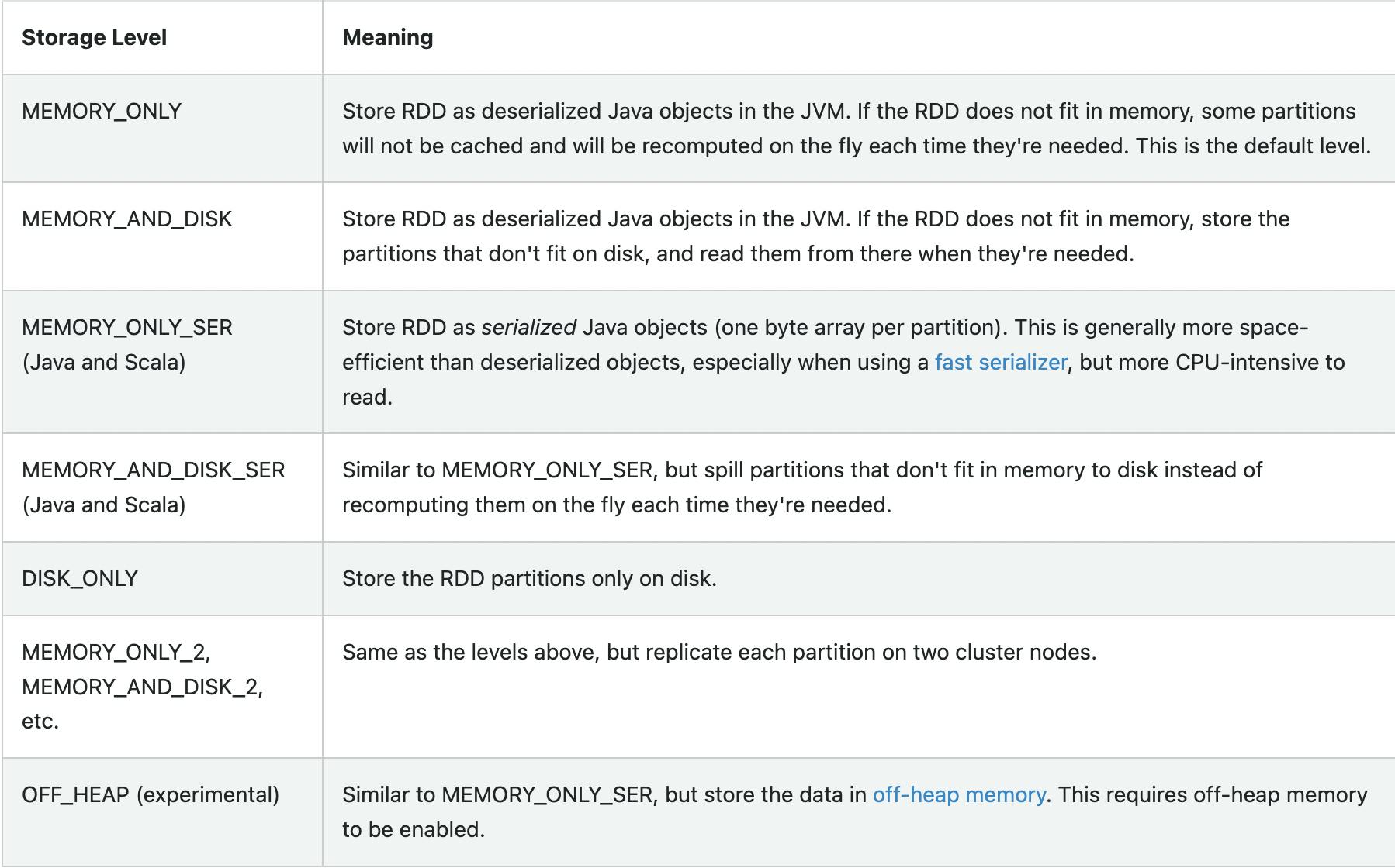
Persisting is similar to caching, but it allows users to choose the storage level for persisted data. Spark provides various storage levels, such as MEMORY_ONLY, MEMORY_ONLY_SER, MEMORY_AND_DISK, MEMORY_AND_DISK_SER, DISK_ONLY, etc. By specifying the storage level, users can control the tradeoff between memory usage and disk space usage.

Keep in mind that caching and persisting data can increase memory usage and potentially cause OutOfMemoryError if you cache too much data. Therefore, it's essential to manage the cache and persist properly and make sure to uncache or unpersist when you no longer need the data.

OFF_HEAP:-

OFF_HEAP refers to a storage mode where data is stored outside of the JVM heap memory, in a separate native memory area. This mode is particularly useful for large datasets or when the available heap memory is limited.

By default, Spark stores data in the JVM heap memory, which has some limitations. For example, the maximum heap size is limited by the available physical memory, and the garbage collector can cause long pauses in the application if the heap size is too large. In addition, the heap memory is not always efficient for storing large objects, such as arrays or data structures, as it can cause heap fragmentation and reduce memory utilization.

To address these limitations, Spark provides an OFF_HEAP storage mode, where data is stored outside the JVM heap memory in a native memory area managed by the operating system. This mode can be particularly useful when dealing with large datasets or when the application requires a lot of memory for caching or processing.

To use OFF_HEAP storage in Spark, users can set the storage level to MEMORY_OFFHEAP when caching or persisting RDDs or DataFrames. For example, the following code caches an RDD using OFF_HEAP storage:

COPY

val rdd = sc.parallelize(Seq(1, 2, 3))
rdd.persist(StorageLevel.MEMORY_ONLY_OFFHEAP)

Keep in mind that using OFF_HEAP storage can have some drawbacks, such as increased memory allocation time and reduced flexibility in memory management. Also, the OFF_HEAP memory is not subject to garbage collection by the JVM, so it's important to manage it carefully and ensure that it doesn't lead to memory leaks or out-of-memory errors.

Block Eviction:-

Block eviction in Apache Spark refers to the process of removing cached data from memory or disk when the system runs out of space or the data is no longer needed. Block eviction is essential for managing memory resources in Spark and avoiding OutOfMemoryErrors.

In Spark, cached data is organized into partitions, and each partition is stored in a separate block in memory or on disk. When the system needs to free up memory for new data or operations, it selects one or more blocks to evict from the cache. The selection process is based on a block eviction policy, which determines which blocks are evicted first. The default policy in Spark is Least Recently Used (LRU), which evicts the least recently accessed blocks first.

When a block is evicted, its partition is removed from memory or disk, and the corresponding memory or disk space is freed up. If the data is still needed for future operations, Spark can recompute it or reload it from disk if it was stored on disk. If the data is no longer needed, Spark can discard it permanently to free up more space.

Users can control block eviction behavior in Spark by configuring various parameters such as the storage level, block size, and eviction policy. For example, increasing the block size can reduce the number of blocks in the cache and improve eviction performance, but it can also increase the risk of OutOfMemoryErrors. Similarly, changing the eviction policy can affect performance and memory usage, so it's important to choose an appropriate policy based on the workload and available resources.

Overall, block eviction is a critical aspect of memory management in Spark, and understanding how it works and how to configure it properly can help optimize performance and prevent memory-related errors.

rdd.toDebugString:-

In Apache Spark, rdd.toDebugString() is a method that can be used to display the lineage of an RDD (Resilient Distributed Dataset) and its dependencies in a readable format. The lineage is a record of the transformations that were applied to the RDD to derive its current state, and it is used to reconstruct the RDD in case of failure or data loss.

When you call rdd.toDebugString(), Spark prints a multi-line string that shows the RDD's dependencies in a tree-like format. The string includes information such as the RDD's ID, the number of partitions, the list of parent RDDs, and the transformations that were applied to each parent RDD to derive the current RDD.

The toDebugString() method can be useful for understanding the lineage of an RDD and diagnosing issues with your Spark application. For example, if you notice that an RDD has a very long lineage with many transformations, it might be a sign that your application is not optimized for performance and could benefit from rethinking the transformations or partitioning.

mapPartitions():-

apachesparkbook.blogspot.com/2015/11/mappar..